Comparing maps

Code

library(terra)
library(sf)
library(docxtractr)
library(tidyverse)
library(readxl)

Code

area <- list.files("data/umrbpl/", full.names = TRUE, pattern = "shp$") |>
  read_sf() |>
  st_transform(crs = "EPSG:4326")

NGP project

These plots are from a reforestation project (secondary forests) in Upper Marikina. The plots are circular and 0.0079 ha in size. In 5-m radius subplots, all trees 5 to 20 cm DBH are measured; in 10-m radius subplots, all trees > 20 cm DBH are measured.

Code

# NGP project
ngp <- list.files("data/inventories/", "NGP", full.names = TRUE) |>
  read_docx() |>
  docx_extract_tbl(1) |>
  set_names(c(
    "plot",
    paste0(rep(c("agb", "agc"), 2), rep(c("_h", ""), each = 2))
  )) |>
  filter(!grepl("Average|Transect", plot)) |>
  mutate(plot = paste0(rep(c(1:23, 27), each = 3), "_", rep(1:3, 24))) |>
  mutate(across(contains("ag"), function(x) {
    ifelse(is.na(as.numeric(x)), 0, as.numeric(x))
  }))

location_ngp <-
  read_excel("data/inventories/Carbon Stock and Sequestration Data.xlsx",
    sheet = "NGP_Carbon Assessment", range = "B3:E84"
  ) |>
  set_names(c("plot", "x", "y", "elev")) |>
  mutate(transect = rep(1:27, each = 3)) |>
  mutate(plot = paste(transect, plot, sep = "_")) |>
  group_by(transect) |>
  # correct problematic x and y values
  mutate(
    x = ifelse(abs(x - median(x)) > 1e4, median(x), x),
    y = ifelse(abs(y - median(y)) > 1e4, median(y), y)
  )

df_ngp <- left_join(ngp, location_ngp) |>
  separate(plot, c("transect", "plot")) |>
  group_by(transect) |>
  summarise(agb = mean(agb_h), x = round(mean(x)), y = round(mean(y)))
sf_ngp <- df_ngp |>
  st_as_sf(coords = c("x", "y"), crs = 32651) |> # check which CRS was used!!
  st_transform(crs = "EPSG:4326")

df_ngp |>
  ggplot(aes(agb)) +
  geom_histogram() +
  labs(x = "Aboveground biomass density (Mg/ha)") +
  theme_classic()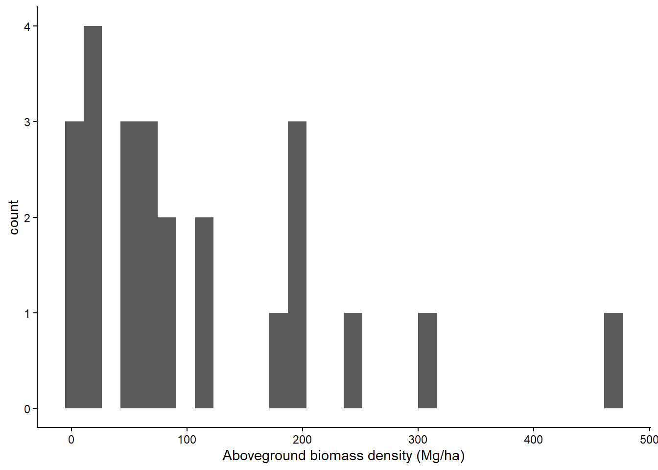

BAMS plots

These are square 20x20m plots.

Code

# BAMS plots
bams <- list.files("data/inventories/", "BAMS", full.names = TRUE) |>
  read_docx() |>
  docx_extract_tbl(1) |>
  set_names(c(
    "plot",
    paste0(rep(c("agb", "agc"), 2), rep(c("_h", ""), each = 2))
  )) |>
  mutate(across(contains("ag"), as.numeric))
location_bams <-
  read_excel("data/inventories/Carbon Stock and Sequestration Data.xlsx",
    sheet = "BAMS_Data", range = "A2:C38"
  ) |>
  rename_with(tolower) |>
  mutate(plot = as.character(rep(1:9, each = 4))) |>
  separate(coordinates, c("x", "y")) |>
  mutate(across(c("x", "y"), as.numeric)) |>
  group_by(plot) |>
  summarise(x = mean(x), y = mean(y))
df_bams <- left_join(bams, location_bams) |>
  select(plot, x, y, agb_h) |>
  rename(agb = agb_h)
df_bams |>
  ggplot(aes(agb)) +
  geom_histogram() +
  labs(x = "Aboveground biomass density (Mg/ha)") +
  theme_classic()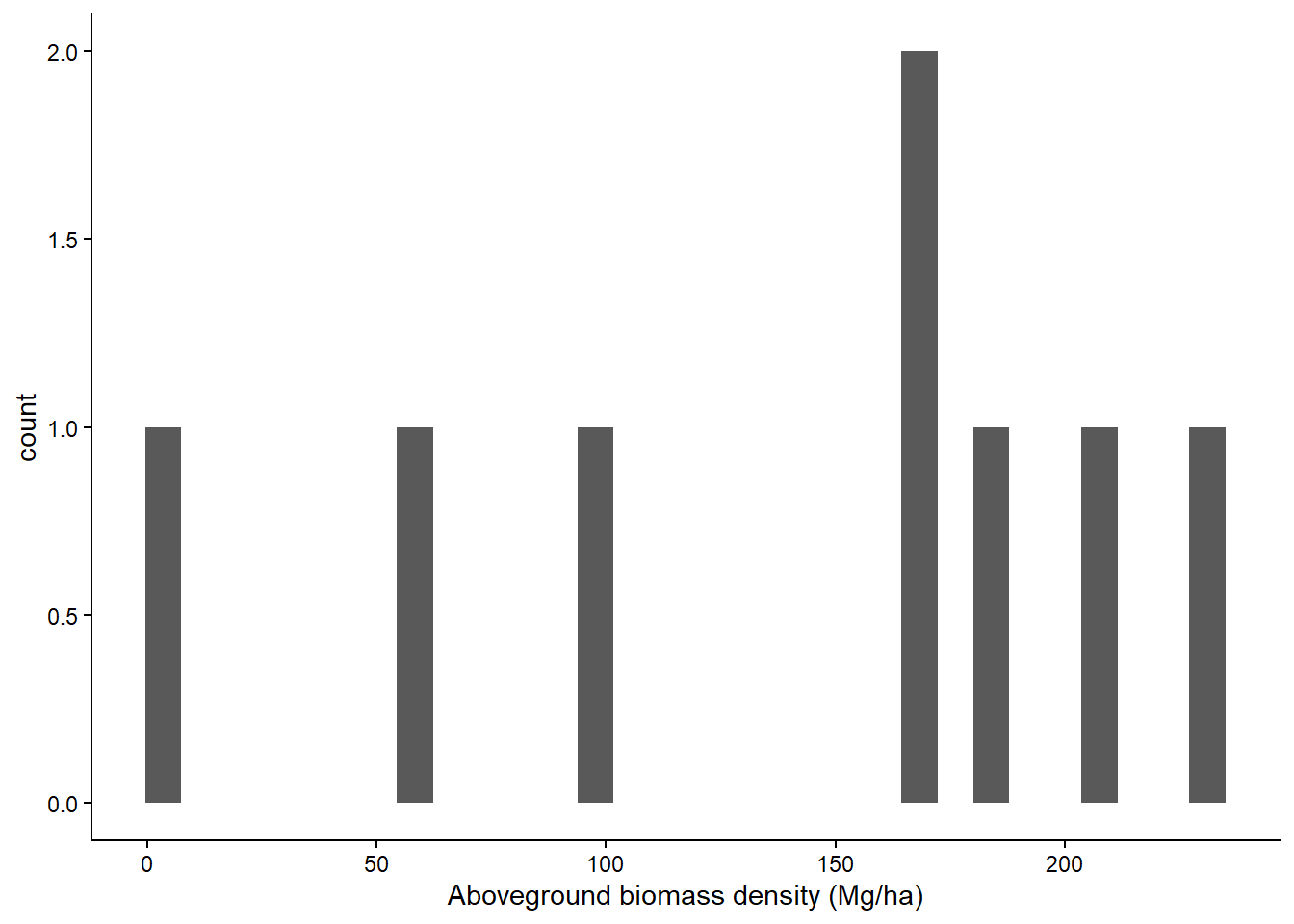

FRA plots

The FRA plots are composed of four 10-m radius plots where all trees >= xx cm DBH are measured, with 5-m nested subplots where all trees >= cm DBH are measured.

Code

fra <- list.files("data/inventories/", "FRA", full.names = TRUE) |>
  read_docx() |>
  docx_extract_tbl(1) |>
  set_names(c(
    "track", "plot",
    paste0(rep(c("agb", "agc"), 2), rep(c("_h", ""), each = 2))
  )) |>
  mutate(across(1:6, as.numeric)) |>
  filter(!is.na(plot)) |>
  fill(track, .direction = "down")
## FRA plots
sf_fra <- st_read("data/inventories/Subplots_Tract105/Subplots_Tract105.shp") |>
  mutate(dataset = "fra") |>
  mutate(plot = paste0("105_", gsub("Plot ", "", PLOT)))

Reading layer `Subplots_Tract105' from data source 
  `D:\github\marikina_carbon\data\inventories\Subplots_Tract105\Subplots_Tract105.shp' 
  using driver `ESRI Shapefile'
Simple feature collection with 4 features and 3 fields
Geometry type: POLYGON
Dimension:     XY
Bounding box:  xmin: 311861.2 ymin: 1631644 xmax: 312383.6 ymax: 1632167
Projected CRS: WGS 84 / UTM zone 51N

Code

fra |>
  ggplot(aes(agb_h)) +
  geom_histogram() +
  geom_vline(xintercept = median(fra$agb_h), lty = 2) +
  annotate(
    geom = "text", x = median(fra$agb_h) + 50, y = 10, angle = 90,
    label = paste("Median:", round(median(fra$agb_h)))
  ) +
  geom_vline(xintercept = mean(fra$agb_h), lty = 2) +
  annotate(
    geom = "text", x = mean(fra$agb_h) + 50, y = 10, angle = 90,
    label = paste("Mean:", round(mean(fra$agb_h)))
  ) +
  labs(x = "Aboveground biomass density (Mg/ha)") +
  theme_classic()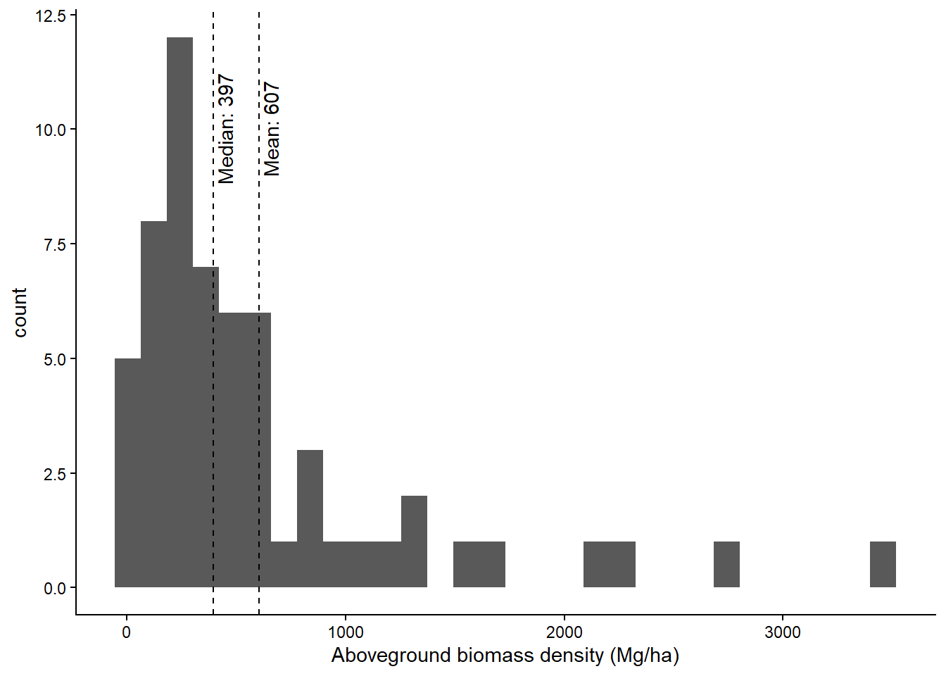

NFI plots

Code

df_nfi <- read.csv("data/inventories/nfi_agb.csv") |>
  mutate(dataset = "nfi") |>
  mutate(plot = paste(tract, plot, sep = "_")) |>
  select(-tract)
location_nfi <- bind_rows(
  read_excel("data/inventories/td.03.xlsx"),
  read.csv("data/inventories/td.14.csv")
) |>
  mutate(plot = paste(tract, plot, sep = "_")) |>
  select(plot, long, lat) |>
  group_by(plot) |>
  summarise(x = median(long), y = median(lat)) |>
  mutate(dataset = "nfi")
df_nfi <- df_nfi |>
  inner_join(location_nfi)

Remove plots classified as non-forest

Code

method <- "tmf"
if (method == "namria") {
  df_nfi$lc <- "data/LULC/egdmis_landcover2015_luzon_20210712/" |>
    list.files("\\.shp", full.names = TRUE) |>
    vect() |>
    terra::extract(df_nfi[, c("x", "y")]) |>
    select(agg12)
  df_nfi |>
    mutate(forest = !is.na(lc) & grepl("forest", tolower(lc$agg12))) |>
    select(-lc) |>
    write.csv("data/inventories/df_nfi.csv", row.names = FALSE)
} else if (method == "tmf") {
  for (yr in c("2003", "2014")) {
    for (coord1 in c("N20", "N10")) {
      for (coord2 in c("E110", "E120")) {
        file <- paste0(
          "data/tmf/JRC_TMF_AnnualChange_v1_", yr,
          "_ASI_ID76_", coord1, "_", coord2, ".tif"
        )
        if (!file.exists(file)) {
          paste0(
            "https://ies-ows.jrc.ec.europa.eu/iforce/tmf_v1/download.py?",
            "type=tile&dataset=AnnualChange_", yr, "&lat=",
            coord1, "&lon=", coord2
          ) |>
            download.file(file, mode = "wb", method = "curl")
        }
      }
    }
  }
  tmf03 <- list.files("data/tmf/", "2003", full.names = TRUE) |>
    grep(pattern = "_N", value = TRUE) |>
    lapply(rast) |>
    sprc() |>
    mosaic()
  tmf14 <- list.files("data/tmf/", "2014", full.names = TRUE) |>
    grep(pattern = "_N", value = TRUE) |>
    lapply(rast) |>
    sprc() |>
    mosaic()
  df_nfi |>
    mutate(
      tmf03 = terra::extract(tmf03, df_nfi[, c("x", "y")])$Dec2003,
      tmf14 = terra::extract(tmf14, df_nfi[, c("x", "y")])$Dec2014
    ) |>
    mutate(tmf = ifelse(year == 2003, tmf03, tmf14)) |>
    mutate(forest = tmf %in% c(1, 2, 4)) |>
    select(plot, year, x, y, forest) |>
    write.csv("data/inventories/nfi_forest.csv", row.names = FALSE)
}

Climate classification

Code

clim <- rast("data/chelsa/climate_variables.tif") |>
  terra::extract(location_nfi[, c("x", "y")], xy = TRUE) |>
  select(-ID) |>
  mutate(plot = location_nfi$plot)
clim$cluster <-
  kmeans(
    scale(clim[, names(rast("data/chelsa/climate_variables.tif"))]),
    3, 25
  )$cluster
# convex hull of upper marikina climate
area <- list.files("data/umrbpl/", full.names = TRUE, pattern = "shp$") |>
  read_sf() |>
  st_transform(crs = "EPSG:4326")
umrbpl <- rast("data/chelsa/climate_variables.tif") |>
  crop(area) |>
  mask(area) |>
  values() |>
  data.frame() |>
  drop_na()
hull_idx <- chull(umrbpl$mean_temperature, umrbpl$mean_precipitation)
hull_idx <- c(hull_idx, hull_idx[1]) # close the polygon
hull <- umrbpl[hull_idx, ]

clim$inside <- sp::point.in.polygon(
  clim$mean_temperature, clim$mean_precipitation,
  hull$mean_temperature, hull$mean_precipitation
)
mutate(clim, inside = inside > 0) |>
  select(plot, inside) |>
  write.csv(file = "data/inventories/nfi_clim.csv", row.names = FALSE)

Code

df_nfi <- df_nfi |>
  select(-x, -y) |>
  inner_join(read.csv("data/inventories/nfi_forest.csv")) |>
  inner_join(read.csv("data/inventories/nfi_clim.csv")) |>
  filter(forest & inside)

Location of the plots

Code

df_fra <- fra |>
  mutate(dataset = "fra", plot = paste(track, plot, sep = "_")) |>
  select(dataset, plot, agb_h) |>
  rename(agb = agb_h) |>
  subset(grepl("105", plot))
df_all <- df_ngp |>
  rename(plot = transect) |>
  mutate(dataset = "ngp") |>
  bind_rows(mutate(df_bams, dataset = "bams")) |>
  bind_rows(select(df_nfi, dataset, year, plot, agb)) |>
  bind_rows(df_fra) |>
  select(-x, -y)
location_ngp <- df_ngp |>
  select(transect, x, y) |>
  rename(plot = transect)
sf_all <-
  bind_rows(list(ngp = location_ngp, bams = location_bams), .id = "dataset") |>
  st_as_sf(coords = c("x", "y"), crs = 32651) |> # check which CRS was used!!
  bind_rows(sf_fra) |>
  st_transform(crs = "EPSG:4326") |>
  bind_rows(st_as_sf(location_nfi, coords = c("x", "y"), crs = 4326))
# within UM
g1 <- ggplot() +
  geom_sf(data = area) +
  geom_sf(
    data = st_crop(sf_all, area),
    aes(col = toupper(dataset), fill = toupper(dataset))
  ) +
  theme_bw() +
  labs(col = NULL, fill = NULL) +
  theme(
    panel.grid = element_blank(),
    axis.text.x = element_text(angle = 45, hjust = 1, vjust = 1),
    legend.position = "none"
  )
g2 <- ggplot(df_all) +
  geom_histogram(aes(x = agb, fill = toupper(dataset))) +
  labs(fill = NULL, y = "Number of plots", x = "AGB (Mg/ha)") +
  theme_bw() +
  theme(
    panel.grid = element_blank(),
    axis.text.x = element_text(angle = 45, hjust = 1, vjust = 1)
  )
ggpubr::ggarrange(g1, g2, labels = c("a", "b"), widths = c(1.2, 2))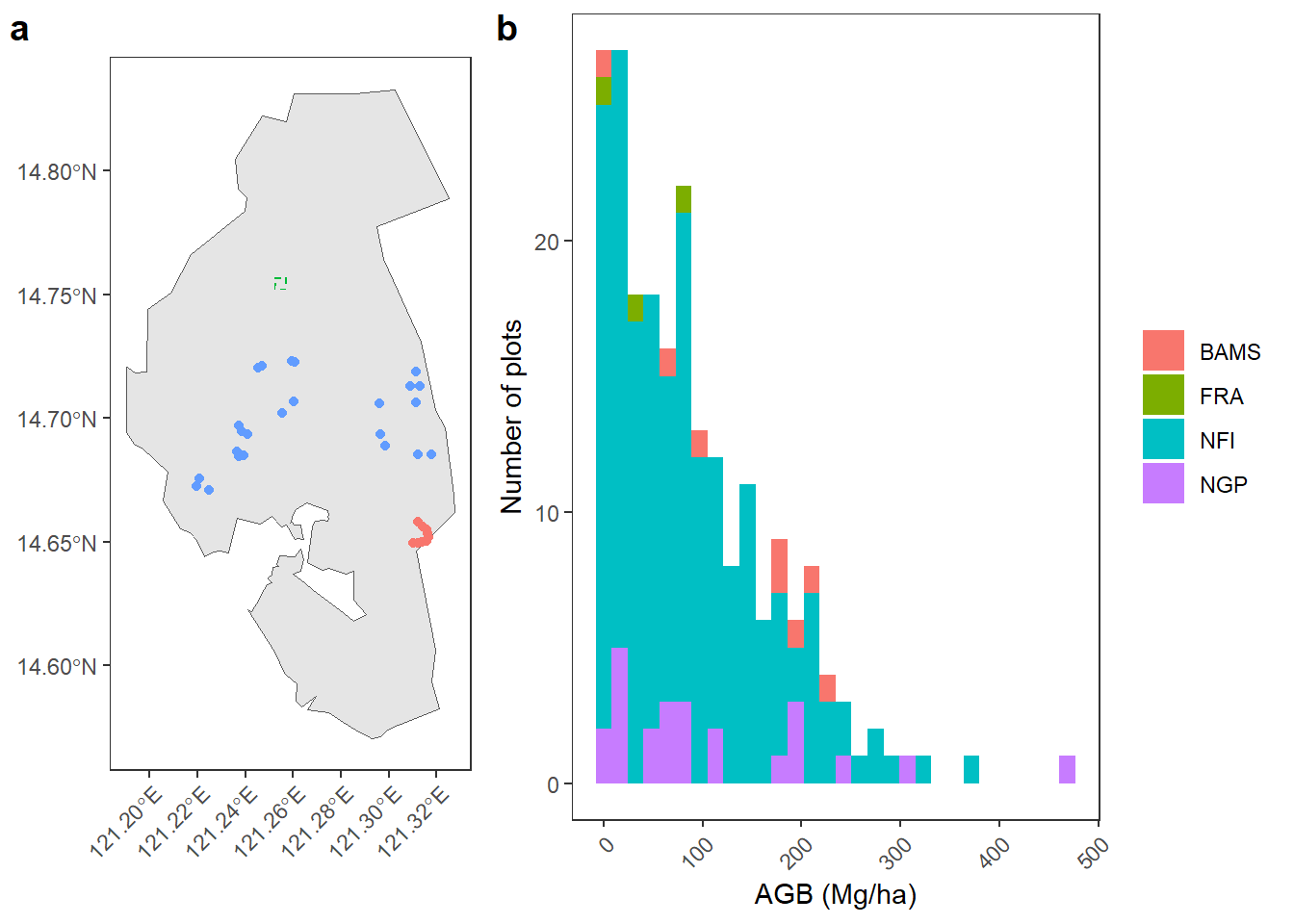

Code

# NFI
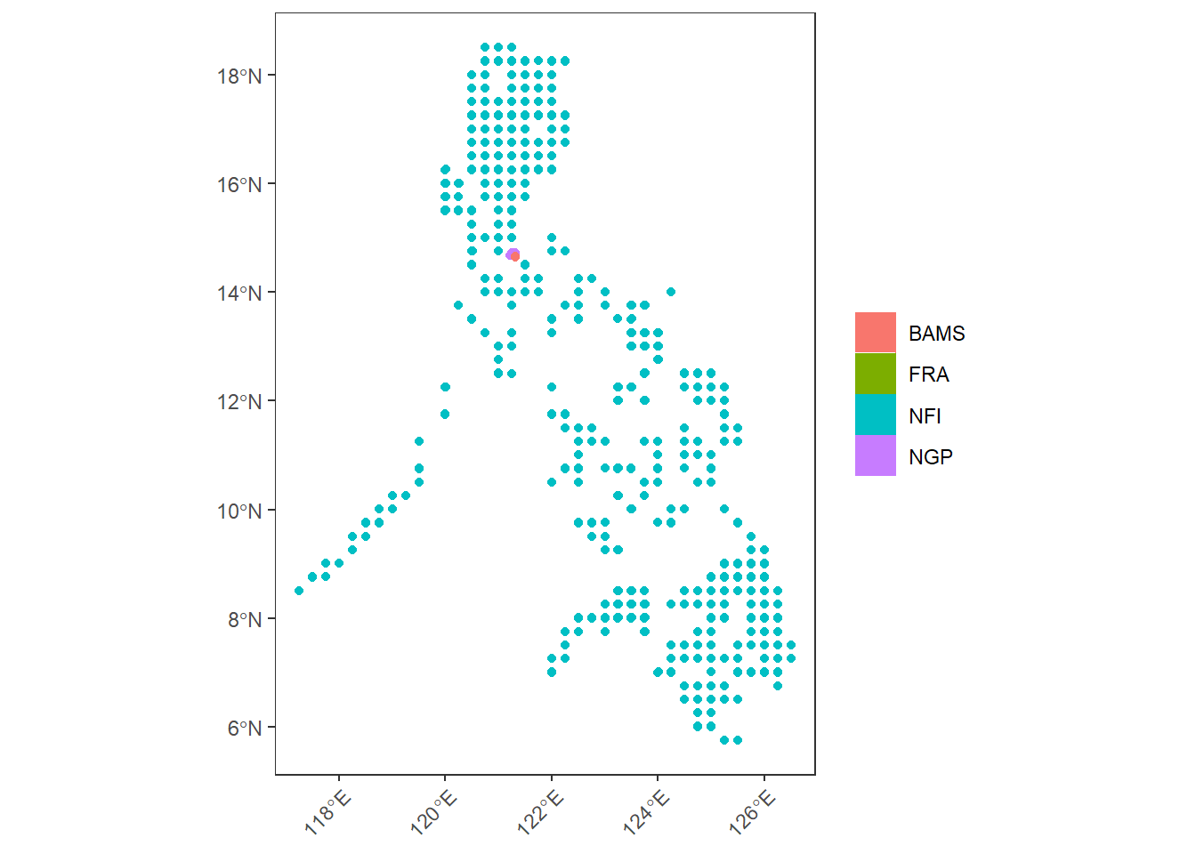
sf_all |>
  ggplot() +
  geom_sf(aes(col = toupper(dataset), fill = toupper(dataset))) +
  theme_bw() +
  labs(col = NULL, fill = NULL) +
  theme(
    panel.grid = element_blank(),
    axis.text.x = element_text(angle = 45, hjust = 1, vjust = 1)
  )

Code

df_all |>
  ggplot(aes(agb, fill = dataset)) +
  geom_density(alpha = 0.6, col = NA) +
  theme_classic() +
  labs(x = "AGB (Mg/ha)")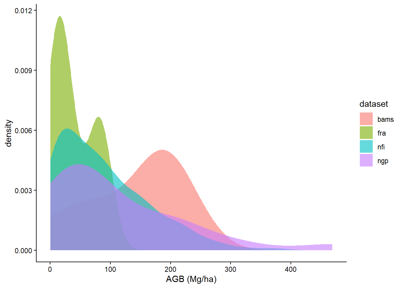

Comparison with biomass maps

Code

df_all <- df_all |>
  filter(dataset != "nfi")

Code

diagnostic <- function(x, y) {
  rmse <- signif(sqrt(mean((x - y)^2, na.rm = TRUE)), 3)
  mape <- signif(mean(abs((x - y) / y), na.rm = TRUE) * 100, 3)
  r2 <- signif(cor(x, y, use = "complete.obs")^2, 2)
  bias <- signif(mean(x - y, na.rm = TRUE), 3)
  cat(
    "RMSE:", rmse,
    "Mg/ha\nMAPE:", mape,
    "%\nR²:", r2, "\nBias:",
    bias, "Mg/ha"
  )
}

Code

robust_extract <- function(coord, rst) {
  if (nrow(coord) > 0) {
    val <- terra::extract(rst, coord)[, 2] |> mean()
  } else {
    val <- NA
  }
}

CCI maps

We match the year of the inventory to the closest year of the map.

Code

cci <- list.files("data/biomass/", "N20E120_ESACCI", full.names = TRUE) |>
  rast()
names(cci) <- do.call(cbind, strsplit(names(cci), "-"))[7, ]

# check inventory year
df_all <- mutate(df_all, year = as.numeric(ifelse(is.na(year), 2010, year)))
df_all$cci_carbon <- sapply(seq_len(nrow(df_all)), function(i) {
  closest <- which.min(abs(as.numeric(names(cci)) - df_all$year[i]))
  sf_all |>
    filter(dataset == df_all$dataset[i] & plot == df_all$plot[i]) |>
    robust_extract(cci[[closest]])
})
diagnostic(df_all$cci_carbon, df_all$agb)

RMSE: 107 Mg/ha
MAPE: 158 %
R²: 0.095 
Bias: -41 Mg/ha

Global forest watch map

Code

gfw <- list.files("data/biomass/", "harris", full.names = TRUE) |>
  rast()
df_all$gfw_carbon <- sapply(seq_len(nrow(df_all)), function(i) {
  sf_all |>
    filter(dataset == df_all$dataset[i] & plot == df_all$plot[i]) |>
    robust_extract(gfw)
})
diagnostic(df_all$gfw_carbon, df_all$agb)

RMSE: 127 Mg/ha
MAPE: 573 %
R²: 0.14 
Bias: 57.4 Mg/ha

GlobBiomass map

Code

glob <- list.files("data/biomass/N40E100_agb/", "agb\\.", full.names = TRUE) |>
  rast()
df_all$glob_carbon <- sapply(seq_len(nrow(df_all)), function(i) {
  sf_all |>
    filter(dataset == df_all$dataset[i] & plot == df_all$plot[i]) |>
    robust_extract(glob)
})
diagnostic(df_all$glob_carbon, df_all$agb)

RMSE: 109 Mg/ha
MAPE: 356 %
R²: 0.019 
Bias: -21.1 Mg/ha

GEDI L4B gridded biomass map

Code

gedi <- rast("data/biomass/GEDI04_B_philippines.tif")[[2]]
df_all$gedi_carbon <- sapply(seq_len(nrow(df_all)), function(i) {
  sf_all |>
    filter(dataset == df_all$dataset[i] & plot == df_all$plot[i]) |>
    robust_extract(gedi)
})
diagnostic(df_all$gedi_carbon, df_all$agb)

RMSE: 120 Mg/ha
MAPE: 423 %
R²: 0.0058 
Bias: -24.5 Mg/ha

Araza map

Code

phmap <- "data/biomass/agb_ph_2015_rf_tc10masked.tif" |>
  rast()
df_all$ph_carbon <- sapply(seq_len(nrow(df_all)), function(i) {
  sf_all |>
    filter(dataset == df_all$dataset[i] & plot == df_all$plot[i]) |>
    robust_extract(phmap)
})
diagnostic(df_all$ph_carbon, df_all$agb)

RMSE: 103 Mg/ha
MAPE: 601 %
R²: 0.18 
Bias: 65.9 Mg/ha

Map choice

Code

map_labs <- c(
  "cci" = "CCI Biomass", "gfw" = "GFW",
  "glob" = "GlobBiomass", "ph" = "Araza",
  "gedi" = "GEDI L4B"
)
df_all |>
  pivot_longer(cols = contains("_carbon")) |>
  filter(!is.na(value)) |>
  mutate(name = gsub("_carbon", "", name)) |>
  ggplot(aes(agb, value)) +
  geom_point(aes(col = toupper(dataset))) +
  facet_wrap(~name, labeller = as_labeller(map_labs)) +
  labs(
    x = "Ground-based AGB (Mg/ha)", y = "Remote-sensing AGB (Mg/ha)",
    col = "Dataset"
  ) +
  geom_abline(slope = 1, intercept = 0, lty = 2) +
  coord_equal() +
  theme_bw() +
  theme(legend.position = "inside", legend.position.inside = c(0.8, 0.25))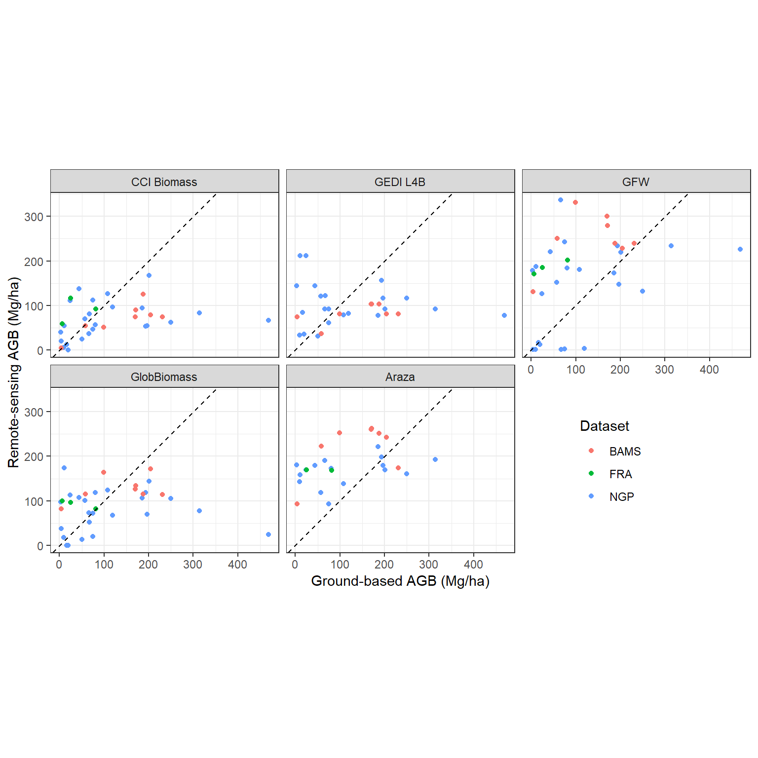

Code

df_all |>
  pivot_longer(cols = contains("carbon"), names_to = "map") |>
  group_by(map) |>
  summarise(
    rmse = signif(sqrt(mean((value - agb)^2, na.rm = TRUE)), 3),
    mape = signif(mean(abs((value - agb) / agb), na.rm = TRUE) * 100, 3),
    r2 = signif(cor(value, agb, use = "complete.obs")^2, 2),
    bias = signif(mean(value - agb, na.rm = TRUE), 3)
  ) |>
  write.csv("C:/Users/piponiot-laroche/Downloads/metrics.csv",
    row.names = FALSE
  )

Compare reference values for biomass in old-growth forests with maps

Code

namria_closed <- "data/LULC/2020_Land Cover/2020_Land Cover_UMRBPL.shp" |>
  read_sf() |>
  filter(CLASS_NAME == "Closed Forest") |>
  st_transform(4326)

cci <- 
  "data/biomass/umrbpl_ESACCI-BIOMASS-L4-AGB-MERGED-100m-2020-fv6.0.tiff" |>
  rast() |> crop(namria_closed) |> mask(namria_closed)
gfw <- rast("data/biomass/harris_carbon_2000.tif") |> 
  crop(namria_closed) |> mask(namria_closed)
arnan <- rast("data/biomass/agb_ph_2015_rf_tc10masked.tif")[[1]] |>
  crop(namria_closed) |> mask(namria_closed)
gedi <- rast("data/biomass/GEDI04_B_philippines.tif")[[2]] |>
  crop(namria_closed) |> mask(namria_closed)
coords <- data.frame(
  lon = runif(1e4, ext(namria_closed)[1], ext(namria_closed)[2]),
  lat = runif(1e4, ext(namria_closed)[3], ext(namria_closed)[4])
)
list("cci", "gfw", "arnan", "gedi") |>
  lapply(function(nmrast) {
    terra::extract(get(nmrast), coords, xy = TRUE)[, 2:4] |>
      set_names("agb", "x", "y") |>
      mutate(map = nmrast)
  }) |> bind_rows() |> drop_na() |>
  ggplot(aes(agb, fill = map)) +
  geom_density(alpha = 0.6, col = NA) +
  labs(x = "AGB (Mg/ha)", y = NULL,
       title = "Distribution of AGB values in pixels classified
       as 'Closed forests' in NAMRIA map") +
  theme_classic()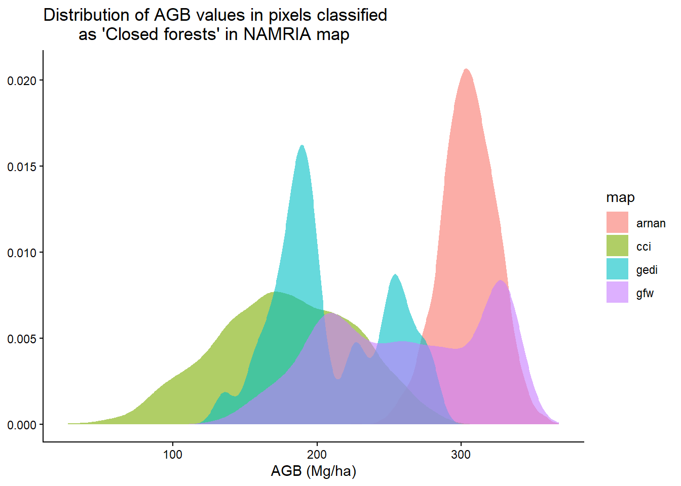

The final map chosen is …