ESA-CCI biomass project

Code

library(sf)
library(terra)
library(ggplot2)
library(tidyterra)
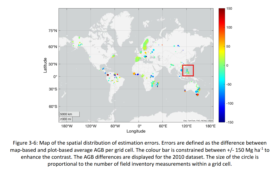
library(dplyr)

The maps are 100-meter resolution, global aboveground biomass maps produced by the European Space Agency’s (ESA) Climate Change Initiative (CCI). These products are based on data from the ESA’s C-band (Sentinel-1A and -1B) and the JAXA’s L-band Synthetic Aperture Radar (ALOS-2 PALSAR-2), as well as additional information from spaceborne lidar (e.g., NASA’s Global Ecosystem Dynamics Investigation Lidar, or GEDI).

According to their validation protocol, they have a substantial validation dataset in the Philippines.

Data

Code

if (!dir.exists("data/biomass")) dir.create("data/biomass")
u0 <- "https://dap.ceda.ac.uk/neodc/esacci/biomass/data/agb/maps/v6.0/geotiff/"
for (year in c(2007, 2010, 2015, 2016, 2017, 2018, 2019, 2020, 2021, 2022)) {
  for (var in c("AGB", "AGB_SD")) {
    url1 <- paste0(
      u0, year, "/N20E120_ESACCI-BIOMASS-L4-", var,
      "-MERGED-100m-", year, "-fv6.0.tif?download=1"
    )
    path1 <- paste0(
      "data/biomass/N20E120_ESACCI-BIOMASS-L4-", var,
      "-MERGED-100m-", year, "-fv6.0.tiff"
    )
    file1 <- paste0(
      "data/biomass/umrbpl_ESACCI-BIOMASS-L4-", var,
      "-MERGED-100m-", year, "-fv6.0.tiff"
    )
    if (!file.exists(file1)) {
      download.file(url1, path1, method = "curl")
      path1 |>
        rast() |>
        crop(ext(121, 121.4, 14.5, 14.9)) |>
        writeRaster(file1)
      file.remove(path1)
    }
  }
}

Code

area <- list.files("data/umrbpl/", full.names = TRUE, pattern = "shp$") |>
  read_sf() |>
  st_transform(crs = "EPSG:4326")
agb <- list.files("data/biomass/", full.names = TRUE) |>
  grep(pattern = "umrbpl", value = TRUE) |>
  grep(pattern = "AGB-", value = TRUE) |>
  rast() |>
  crop(ext(area)) |>
  mask(area) |>
  tidyterra::rename_with(~ sapply(strsplit(.x, "-"), function(i) i[7]))
uncertainty <- list.files("data/biomass/", full.names = TRUE) |>
  grep(pattern = "umrbpl", value = TRUE) |>
  grep(pattern = "AGB_SD", value = TRUE) |>
  rast() |>
  crop(ext(area)) |>
  mask(area) |>
  tidyterra::rename_with(~ sapply(strsplit(.x, "-"), function(i) i[7]))
ggplot() +
  geom_spatraster(data = agb) +
  facet_wrap(~lyr, nrow = 2) +
  scale_fill_viridis_c("AGB\n(Mg/ha)")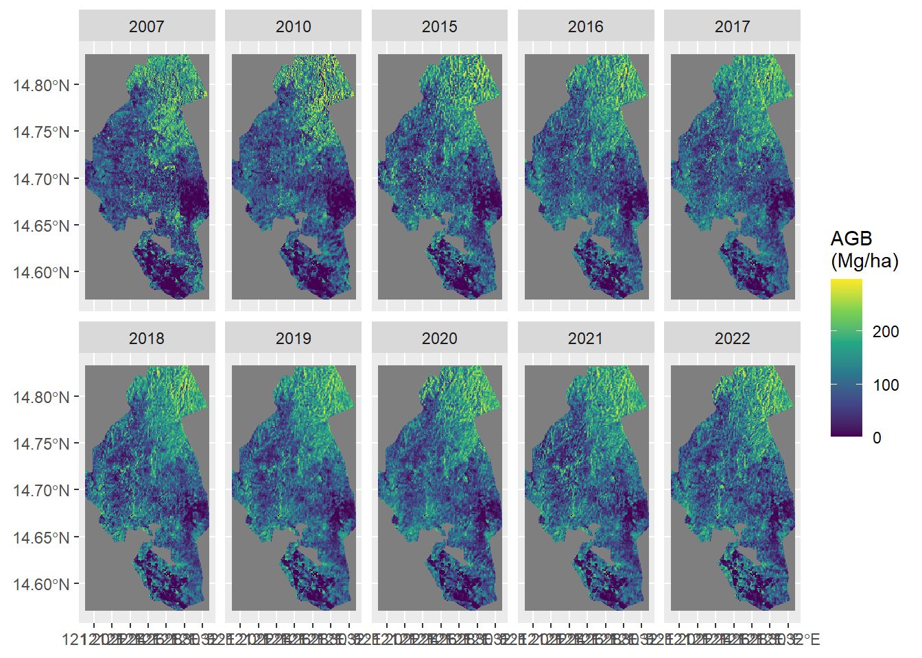

Code

ggplot() +
  geom_spatraster(data = uncertainty / agb * 100) +
  facet_wrap(~lyr, nrow = 2) +
  scale_fill_viridis_c("Coefficient of variation (%)", option = "magma")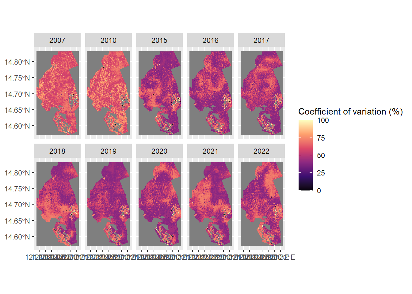

Distribution of AGB by TMF class

Code

tmf <- list.files("data/tmf", "UMRBPL", full.names = TRUE) |>
  rast() |>
  crop(area) |>
  mask(area)
agb <- resample(agb, tmf, method = "average")

df_tmf <- as.data.frame(tmf, xy = TRUE) |>
  pivot_longer(
    cols = matches("19|20"),
    names_to = "year", values_to = "class"
  ) |>
  mutate(year = gsub("Dec", "", year)) |>
  filter(class != 0)
df_tmf$class <- factor(df_tmf$class)
levels(df_tmf$class) <- c(
  "Undisturbed", "Degraded", "Deforested",
  "Regrowth", "Water", "Other"
)
df_agb <- as.data.frame(agb, xy = TRUE) |>
  pivot_longer(cols = contains("20"), names_to = "year", values_to = "agb") |>
  inner_join(as.data.frame(cellSize(agb, unit = "ha"), xy = TRUE))
data_all <- inner_join(df_agb, df_tmf)

ggplot(data_all) +
  geom_violin(aes(x = class, y = agb, col = class))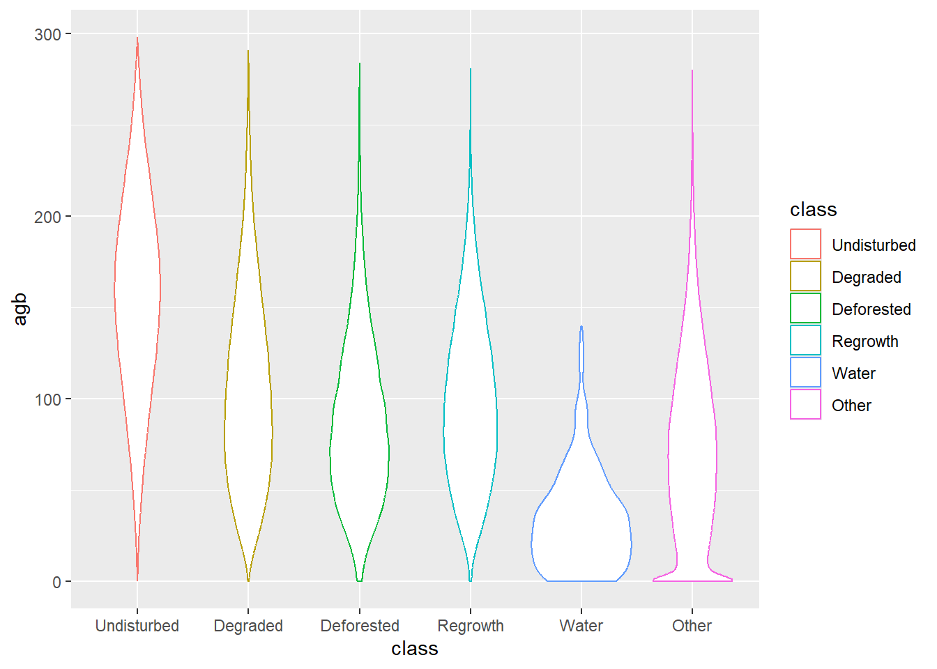

AGB stocks by TMF class through time

Code

data_all |>
  group_by(class, year) |>
  summarise(agbtot = sum(agb * area)) |>
  ggplot(aes(fill = class, y = agbtot, x = as.numeric(year))) +
  geom_bar(position = "stack", stat = "identity") +
  labs(y = "AGB (Mg/ha)", x = "Year") +
  scale_fill_manual(name = "", values = c(
    "Undisturbed" = "darkgreen",
    "Degraded" = "orange",
    "Deforested" = "red",
    "Regrowth" = "green",
    "Water" = "lightblue",
    "Other" = "grey"
  )) +
  theme_classic()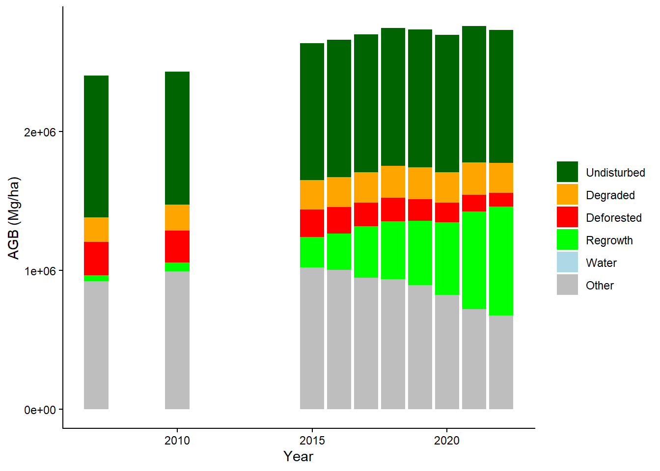

AGB vs secondary forest age (according to TMF)

Only forests marked as secondary:

Code

df_age <- lapply(unique(df_agb$year), function(yr) {
  i <- grep(yr, names(tmf)) # nolint
  tmf_sec_age <- mask(x = tmf[[seq_len(i)]], ifel(tmf[[i]] == 4, 1, NA)) |>
    app(\(x) {
      if (any(!is.na(x) & x != 4)) {
        length(x) - max(which(x != 4))
      } else {
        NA
      }
    })
  as.data.frame(tmf_sec_age, xy = TRUE) |>
    rename(age = lyr.1) |>
    inner_join(filter(df_agb, year == yr))
}) |>
  bind_rows()

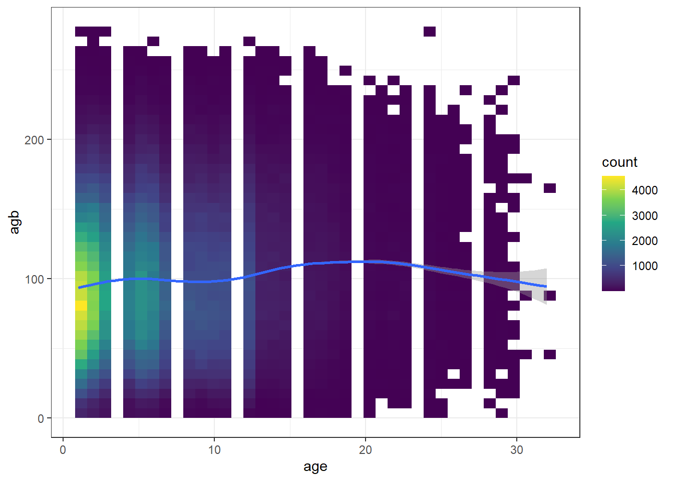
ggplot(df_age, aes(x = age, y = agb)) +
  geom_bin2d(bins = 40) +
  geom_smooth() +
  scale_fill_continuous(type = "viridis") +
  theme_bw()